Logging and Visualization

In this part, we will introduce how to record and save everything you want during an experiments. The contents are organized as follows:

• How to understand the log file after the experiment finished.
• How to visualize with log file after experiment finished.
• How the logging module of Baconian works.

Log Directory Explanation

After one experiment finished, lots of built-in logging information will be recorded and saved to file so you can visualize and analysis the results. A typical logging file directory looks like this:

.
 ├── console.log             # log output to console during experiments
 ├── final_status.json       # final status of all modules when the experiment finished
 ├── global_config.json      # config you use for this experiment include default config and customized config.
 ├── record                  # record folder contains all raw log of experiments.
 │   ├── agent               # agent level log (training samples' reward, test samples' reward etc.)
 │   │   ├── CREATED.json    # agent's log under CREATED status
 │   │   ├── INITED.json     # agent's log after CREATED and into INITED status
 │   │   ├── TRAIN.json      # agent's log under training status (e.g., reward received when sample for training, action during training sampling)
 │   │   └── TEST.json       # agent's log under test status (e.g., reward received when sample for evaluation/test)
 │   └── algo                # algorithm level log (loss, KL divergence, etc.)
 │   │   ├── CREATED.json    # algorithm's log under CREATED status
 │   │   ├── INITED.json     # algorithm's log after CREATED and into INITED status
 │   │   ├── TRAIN.json      # algorithm's log under training status (e.g., training loss)
 │   │   └── TEST.json       # algorithm's log under test status
 └── model_checkpoints       # store the checkpoints of tensorflow models if you have add the saving scheduler in your experiments.

Visualize and analyze the log

Three plot modes: line, scatter and histogram are available within plot_res function in log_data_loader. plotter will use Matplotlib package to plot a graph with data_new DataFrame as input. Users may utilise visualisation.py for fast plotting, with existing single or multiple experiment results.

Please refer to the following examples for single or multiple experiment visualisation:

• Single Experiment Visualisation

We use the log generated by running the Dyna examples as example.

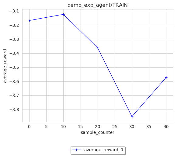
Following code snippet is to draw a line plot of average_reward that agent received during training, using data sampled from environment as index and averaged every 10 rewards for smooth line.

Note

sub_log_dir_name should include the COMPLETE directory in between the log_path directory and json.log. For example, if you have a log folder structured as /path/to/log/record/demo_exp_agent/TEST/log.json, then the sub_log_dir_name should be demo_exp_agent/TEST/ and exp_root_dir should be /path/to/log/.

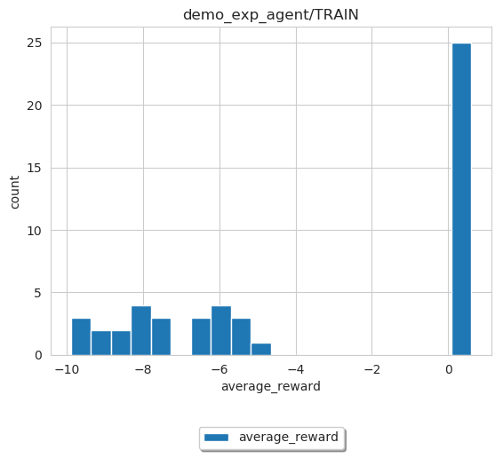
Please note that histogram plot mode is a bit different from the other two modes, in terms of data manipulation. Although index is unnecessary under histogram mode, but currently user still should pass in one for internal data processing.

image = loader.SingleExpLogDataLoader(path)
image.plot_res(sub_log_dir_name='demo_exp_agent/TRAIN',
           key="average_reward",
           index='sample_counter',
           mode='histogram',
           save_format='pdf',
           save_flag=True,
           file_name='average_reward_histogram'
           )

• Multiple Experiment Visualisation

Visualize the results from multiple runs can give a more reliable analysis of the RL methods, by plotting the mean and variance over these results. Such can be done by MultipleExpLogDataLoader

We use the DDPG benchmark experiments as example, use can found the script under the source code baconian-project/baconian/benchmark/run_benchmark.py

Following code snippet is to draw a line plot of sum_reward in benchmark_agent/TEST as a result of 10 times of DDPG benchmark experiments.

path = '/path/to/log' # under the path, there should be 10 sub folders, each contains 1 experiment results.
image = loader.MultipleExpLogDataLoader(path)
image.plot_res(sub_log_dir_name='benchmark_agent/TEST',
               key="sum_reward",
               index='sample_counter',
               mode='line',
               save_flag=True,
               average_over=10,
               save_format='pdf'
               )

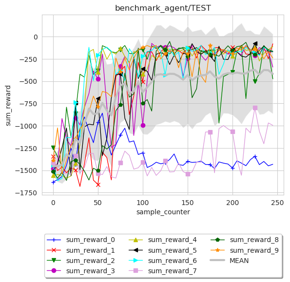
We can see from the results that DDPG is not quite stable as 2 out of 10 runs failed to converge.

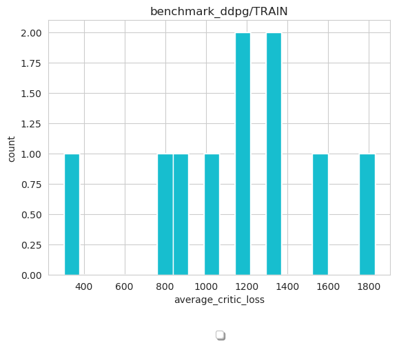
When plotting multiple experiment results in histogram mode, figure will reflect the histogram/data distribution using all experiments’ data.

path = '/path/to/log'
image = loader.MultipleExpLogDataLoader(path)
image.plot_res(sub_log_dir_name='benchmark_ddpg/TRAIN',
               key="average_critic_loss",
               index='train',
               mode='histogram',
               file_name='average_critic_loss_benchmark',
               save_format='pdf',
               save_flag=True,
               )

We can use the action distribution to analyze and diagnose algorithms.

How the logging module of Baconian works

There are two important modules of Baconian: Logger and Recorder, Recorder is coupled with every module or class you want to record something during training or testing, for such as DQN, Agent or Environment. It will record the information like loss, gradient or reward in a way that you specified. While Logger will take charge of these recorded information, group them in a certain way and output them into file, console etc.